InterpretML - Great to have tool 🛠️ in MLOps toolkit 🧰 !

Hi All,

InterpretML is an open-source package by Microsoft that encompasses SOTA ML interpretability techniques. It works for two categories: Glassbox models: The ML models that are designed for interpretability such as linear models, GAMs. Blackbox models: PDP, LIME techniques for explaining existing systems.

Microsoft Research has developed an interpretable model named Explainable Boosting Machine (EBM). It is a GAMs + bagging/boosting (GAMs on steroids!) in simple terms. The link to the paper is here. As mentioned in the paper, EBM is a generalized additive model which learns each feature function f using modern machine learning techniques such as boosting and bagging. EBM can also detect and include pairwise interaction terms as shown.

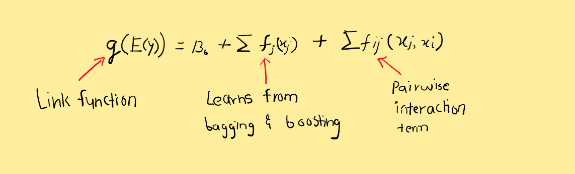
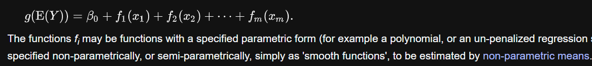
If you see the original definition of GAM from wikipedia, the functions f may be parametric, non-parametric, or semi-parametric (smooth functions).

Let’s import the required libraries and datasets. I am using the same datasets that I have been using for the last few articles. The dataset is available at Kaggle. It is a simple classification example to predict whether a customer will change telco provider. I faced a setback while using interpret in python scripting (.py), so I used .ipynb for the scripting.

import numpy as np
import ipykernel as ipy
import pandas as pd
import yaml
import argparse
import typing
import matplotlib.pyplot as plt
from sklearn.metrics import f1_score,recall_score,accuracy_score,precision_score,confusion_matrix,classification_report
from interpret.glassbox import ExplainableBoostingClassifier
from interpret import show
from interpret.provider import InlineProvider
from interpret import set_visualize_provider
set_visualize_provider(InlineProvider())
from interpret.data import ClassHistogram
from interpret import show, preserve, show_link, set_show_addr

Import the train, test datasets, and split them into independent and dependent.

df = pd.read_csv('C:\\Users\\ashis\\OneDrive\\Desktop\\MLOps\\churn_model\\data\\processed\\churn_train.csv')
df_test = pd.read_csv('C:\\Users\\ashis\\OneDrive\\Desktop\\MLOps\\churn_model\\data\\processed\\churn_test.csv')
df.head()

train_x = df[[col for col in df.columns if col not in ['churn']]]
train_y = df['churn']
test_x = df_test[[col for col in df_test.columns if col not in ['churn']]]
test_y = df_test['churn']

print(f'train shape: {train_x.shape}')
print(f'test shape: {test_x.shape}')

Build a EBC and try a global explainability on the trained model. I had the set-up IP address and port number as the default address was different.

# Fit an Explainable Boosting Machine
ebm = ExplainableBoostingClassifier()
ebm.fit(train_x, train_y)

ebm_global = ebm.explain_global(name = 'EBM')
#preserve(ebm_global, 'number_customer_service_calls', 'number_customer_service_calls.html')
set_show_addr(("127.0.0.1", 5000))
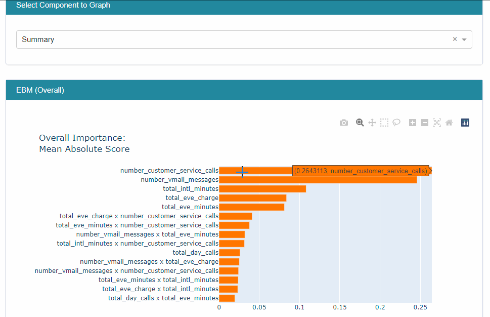
show(ebm_global)

The result is a plotly interactive graph. I created a gif to show various options available. When we select ‘summary’ option in the dropdown, it gives overall feature importance. The feature ‘number_customer_service_calls’ has the maximum feature importance. When we select ‘number_customer_service_calls’ in the dropdown, it gives a score for a complete feature range. As the ‘number_customer_service_calls’ value increases, the score also increases, i.e., higher chances of churning.

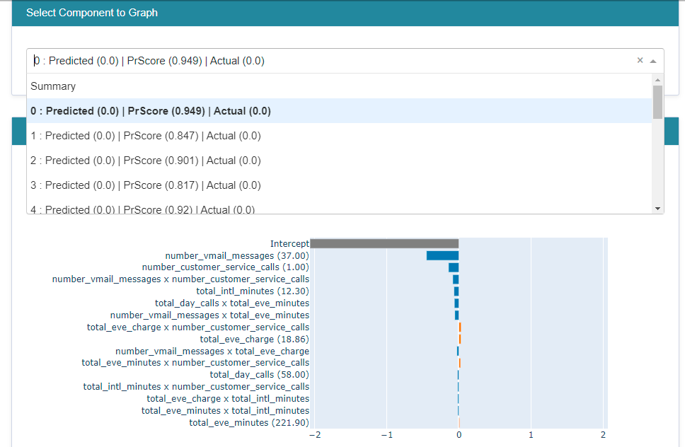
The local explainability for a few records can be examined for a better understood as

ebm_local = ebm.explain_local(train_x[:20], train_y[:20], name='EBM')
show(ebm_local)

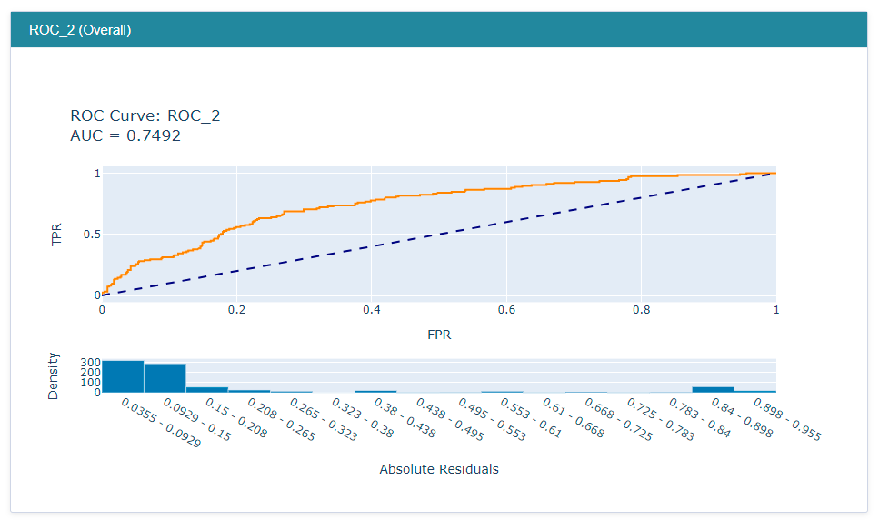
The ROC performance can be accessed for the best model after the hyperparameter tuning by running below code:

from interpret.glassbox import ExplainableBoostingClassifier
from sklearn.model_selection import RandomizedSearchCV
param_test = {'learning_rate': [0.001,0.005,0.01,0.02],
              'interactions': [5,10,15],
              'max_interaction_bins': [10,15,20],
              'max_rounds': [500,1000,1500,2000],
              'min_samples_leaf': [2,3,5],
              'max_leaves': [3,5,10]}
n_HP_points_to_test=10
LGBM_clf = ExplainableBoostingClassifier(random_state=314, n_jobs=-1)
LGBM_gs = RandomizedSearchCV(
    estimator=LGBM_clf,
    param_distributions=param_test,
    n_iter=n_HP_points_to_test,
    scoring="roc_auc",
    cv=3,
    refit=True,
    random_state=314,
    verbose=False,
)
LGBM_gs.fit(train_x, train_y)

from interpret import perf
roc = perf.ROC(LGBM_gs.best_estimator_.predict_proba, feature_names=train_x.columns)
test_y = test_y.map({'yes':1,'no':0})
roc_explanation = roc.explain_perf(test_x, test_y)
show(roc_explanation)

I think InterpretML can be a really important part of MLOps pipeline!! Sorry, Missed to mentioned and want to give a big shoutout to Cockos for providing a lightweight tool for gif creation.