Coastline Zip Codes (USA) - New Approach

The last blog gives an approach to find the coastline zip codes. I followed the relative distances calculation approach to find the zip codes. I came across ‘Natural Earth’ and an R package ‘rnaturalearth’ which is the API to the site.

The piece of code gives the Latitude and Longitude coordinates of the coastline zip codes:

library(tidyverse)
library(sf)
library(raster)
library(rnaturalearth)
library(rgeos)

USA <- ne_countries(scale = 110, 
                    country = "United States of America", 
                    returnclass = "sf")
USA_lat_long <- st_transform(USA, 
                             "+proj=longlat +ellps=WGS84 +datum=WGS84")
USA_df_lat <- st_coordinates(USA_lat_long) %>% 
  data.frame() %>% 
  dplyr::rename(long = X, lat = Y) %>% 
  dplyr::select(lat,long)

The CSV file extract is available on my github page to download.

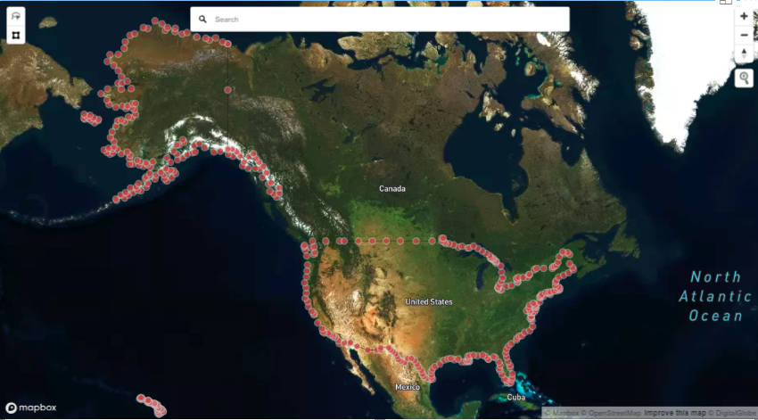
I used Mapbox for map visualization. Below graph shows the coastline boundary (including Alaska).

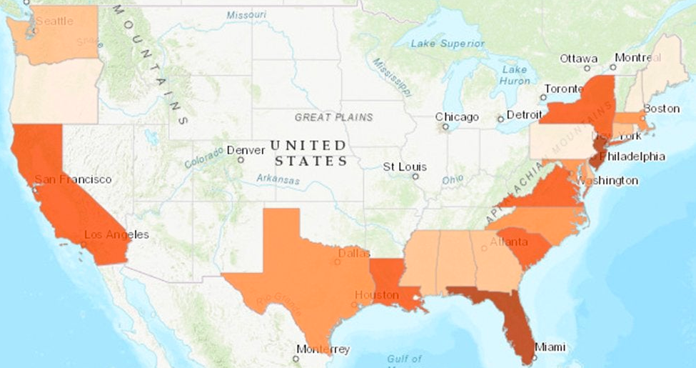
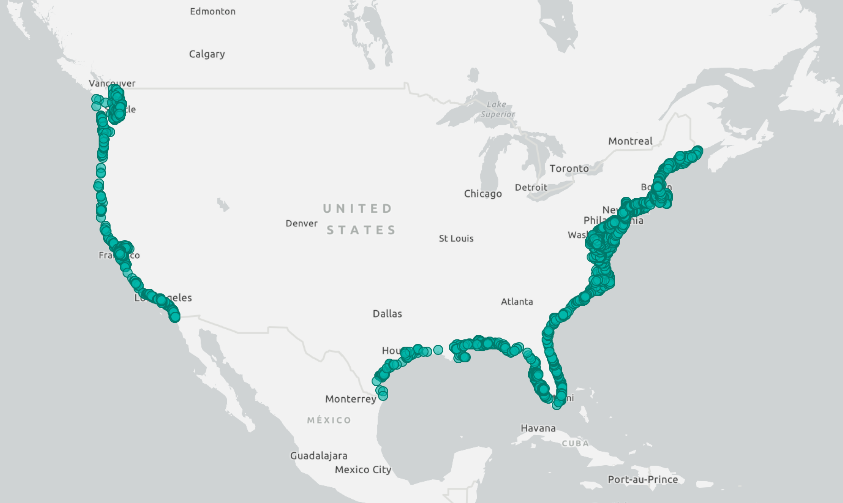
Once I had the coastline lat and long, I wrote SQL query conditioned on lat and long (e.g. lat - 0.02 > zip_lat > lat + 0.02) to fetch the ZIP codes. It gave a good match to pull ZIP codes. The below graph shows the boundary highlighting the ZIP codes (excluding Alaska)

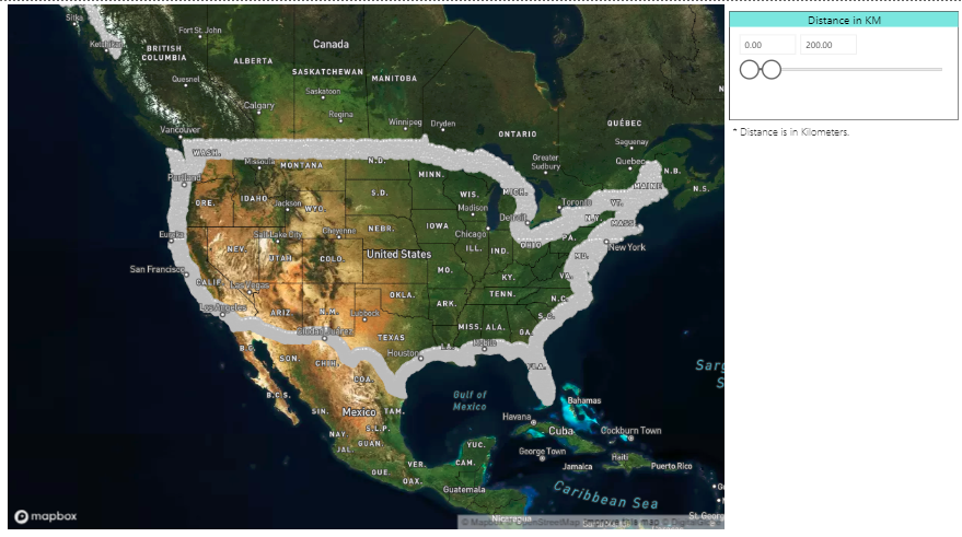
The below piece of code gives the distance in Km from the coastline coordinates. The distance can be used as a filter on the dashboard as shown.

# Distance calculations
USA <- ne_countries(scale = 110, 
                    country = "United States of America", 
                    returnclass = "sf")
proj4string(USA)
USA <- st_transform(USA, 3055)
# Grid formation
grid <- st_make_grid(USA, 
                     cellsize = 50000, 
                     what = "centers")
grid <- st_intersection(grid, USA)
plot(grid)

USA_cast <- st_cast(USA, "MULTILINESTRING")
distance <- st_distance(USA_cast, grid)

df <- data.frame(dist = as.vector(distance)/1000,
                 st_coordinates(grid))


# Converting to required projection (longlat)
dfcoor <- df
coordinates(dfcoor) <- ~X+Y
proj4string(dfcoor) <- CRS("+proj=utm +zone=27 +ellps=intl +towgs84=-73,47,-83,0,0,0,0 +units=m +no_defs")
dfcoor_lat <- spTransform(dfcoor, 
                          CRS("+proj=longlat +ellps=WGS84 +datum=WGS84"))
df_lat <- coordinates(dfcoor_lat) %>% 
  data.frame() %>% 
  rename(long = X, lat = Y)

# Combining the tables
USA_dataset <- cbind(df, df_lat)
write.csv(USA_dataset, "E:\\Study\\Power_BI\\USA_dataset.csv")

The below piece of code gives the distance in Km from the coastline coordinates. The distance can be used as a filter on the dashboard as shown.

The USA_dataset which includes the distance values is available on my github page.

Thank you for reading the post!