Market Mix Modeling using Pycaret and Streamlit (part 1)!!

Hi All,

The holiday break is a great time to learn something new and impactful. As always, I chose technical stuff over the rest 😬. I had two things to explore and use effectively. The first one is the package ‘PyCaret’. As per the documentation, it is an open-source, low-code machine learning python library that automated the machine learning workflows. There are many salient features you can explore.

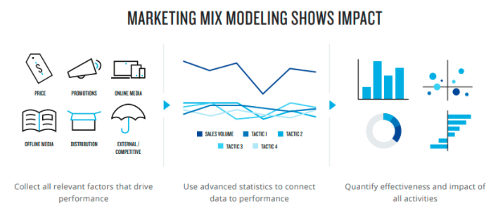
I think the most profound way to explore and learn new things is to apply the new learnings to some business problem. I decided to choose ‘Marketing mix modeling’ for that. Marketing mix modeling (MMM) is a statistical analysis such as multivariate regressions on sales and marketing time series data to estimate the impact of various marketing tactics (marketing mix) on sales and then forecast the impact of future sets of tactics. It is often used to optimize advertising mix and promotional tactics with respect to sales revenue or profit. wiki

The dataset I leveraged for this is Advertising and sales. It is a concise dataset with three independent features and ‘Sales’ as a target variable.

# Loading required packages
import pandas as pd
import numpy as np
import os

path = "D:\Python Files"
file_name = "Advertising.xlsx"
print(os.path.join(path,file_name))

input_file = os.path.join(path,file_name)

# Load the data
def load_data():
    data = pd.read_excel(input_file, engine='openpyxl')
    print(data.shape)
    return data

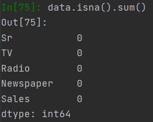
The data does not contain any missing values. The dataset size is (200,5).

Let’s import the required modules of pycaret. We can check the transformations and explore more about the pipeline using ‘get_config()’.

# Importing the pycaret modules
from pycaret.regression import *
from pycaret.utils import version

# Check version
def version_check():
    print(version())
    return None
    
help(get_config)
get_config('prep_pipe')

I set up the function pipeline in the required sequence. As it is a regression modeling problem, we can find the detailed documentation at PyCaret site.

if __name__ == '__main__':
    # Checking version
    version_check()
    data = load_data()

    # check missing values
    data.isna().sum()

    # Data shape
    data.shape

    # column names
    print(data.columns)

    # Setup run
    s = setup(data=data,
              target='Sales',
              ignore_features=['Sr'],
              transformation=True,
              transform_target=True,
              normalize=True)

    lr = create_model('lr')
    tuned_lr = tune_model(lr)

    plot_model(tuned_lr, plot="residuals", save=True)

Let’s discuss each function in detail:

1.version_check(): It just checks the version of PyCaret installed. You can also check the package version in Pycharm as:

File -> Settings -> Python Interpreter -> (Package, Version, Latest version)

2.load_data(): I wrote this function to read the data from an Excel file. We can read the data in any format. There have been a few changes recently for reading the excel files. We can also explore the PyCaret through inbuilt datasets using get_data() function.

3.setup(): As per the Pycaret documentation, this function initializes the training environment and creates the transformation pipeline. We set up the nornmalize parameter to True to apply zscore normalize method. Similarly, we set up the transformation parameter to True to apply yeo-johnson transformation to make data more Gaussian-like. We apply Box-cox transformation to the target variable Sales. The Box-cox transformation is suitable as our data has strictly positive values.

4.create_model(): This function trains and evaluates the performance of Linear Regression (lr) using cross-validation. It returns a trained model.

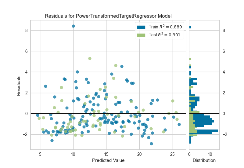
5.plot_model(): It analyzes the performance of a trained model on holdout set. I saved the residuals plot graph by making save parameter True. The plot looks like:

Let’s see the rest of the functions

# Predictions on holdout sample
    pred_holdout = predict_model(tuned_lr)

    # Creating Line Graph
    from matplotlib.pyplot import figure

    figure(num=None, figsize=(15, 6), dpi=80, facecolor='w', edgecolor='k')

    y1 = pred_holdout['Sales']
    y2 = pred_holdout['Label']
    plt.plot(y1, label='Actual')
    plt.plot(y2, label='Predicted')
    plt.legend()
    plt.show()

    final_lr = finalize_model(tuned_lr)

    # saving the model for 'streamlit' app
    save_model(final_lr, 'saved_MMM_lr')

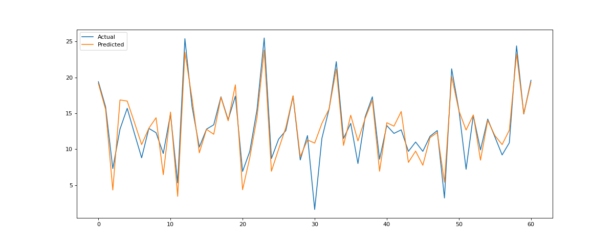
The Actual vs. Predicted values on the holdout sample take the below shape:

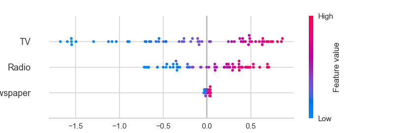
We can even interpret the tree-based model based on SHAP.

6.finalize_model(): It trains Linear Regression on the entire dataset including the holdout set.

7.save_model(): It saves the final model as pickle (.pkl) file with given name.

In the next post, we will see how to create and run streamlit app. The web-based will run on the local system.

Thank you for reading!!